Adding Spatial Information

Goal

This example demonstrates how spatial information can be integrated into an agent-based model using Vahana. While Vahana's primary focus is on graph-based simulations, it support the inclusion of spatial information into models. It allows you to define a spatial grid, associate agents with specific locations, and implement interactions based on spatial proximity, even though the underlying implementation still operates on graph structures.

It's worth noting that in its current version, Vahana may not be the optimal choice for models that primarily depend on frequent movement of agents across space. However, as this example will show, it is entirely possible to implement those models.

It allows you to define a spatial grid, associate agents with specific locations, and implement interactions based on spatial proximity, all while leveraging Vahana's efficient graph-based computations.

For the understanding of how Vahana handles spatial information and rasters, you may find it helpful to watch also the corresponding section of the Vahana.jl Juliacon video. The video provides a visual explanation of how rasters are implemented within Vahana's graph-based framework and demonstrates some key concepts that we'll be applying in this tutorial.

In this tutorial, we'll implement a predator-prey model with spatial components, showcasing how Vahana's raster functionality can be used to create a spatially-explicit ecological simulation.

The model is based on the Predator-Prey for High-Performance Computing (PPHPC) model. In PPHPC the agents move randomly, in our implementation the prey move to locations with grass (if one is in sight) and the predators move to locations with prey to demonstrate how features like this can be implemented in Vahana.

Agent and Edge Types

using CairoMakie, Vahana, Random

true

In our spatial predator-prey model, we define separate structures for predators and prey, even though they share the same fields:

struct Predator
    energy::Int64
    pos::CartesianIndex{2}
end

struct Prey
    energy::Int64
    pos::CartesianIndex{2}
end

Despite their identical structure, we define them as separate types because Vahana uses these types as tags for differentiating between agent categories.

In the following sections, we'll use "Species" as an umbrella term to refer to both Predator and Prey. Functions that are applicable to both types will take the type as a parameter, which we'll denote as Species in the function arguments.

Aside from the predator and prey agents, the spatial environment is represented by grid cells, which are also implemented as agents and consequently function as nodes within the graph structure.

struct Cell
    pos::CartesianIndex{2}
    countdown::Int64
end

All agents maintain their position as part of their internal state. However, a cell can only perceive the animals if they are directly connected to the cell through an edge. Vahana facilitates the establishment of such edges via the move_to! function.

Edges represent connections from prey or predators to cells. We define Position as a parametric type, enabling cells to distinguish between prey and predators based on the type of the edges.

struct Position{T} end

Views are also edges from the cells to the prey and predators respectively. These edges represent the cells that are visible to a prey or predator so that, for example, it is possible to check which cell in the visible area contains food.

struct View{T} end

VisiblePrey edges represent connections from prey to predator. Currently, all edge types link animals to cells, and without an incoming edge from prey, a predator lacks awareness of prey positions. The VisiblePrey edges are generated by cells through the find_prey transition function, as cells possess knowledge of which Prey entities are directly located on the cell via the Position{Prey} edges, and consequently within the view of a predator via the View{Predator} edges.

struct VisiblePrey end

The last two edge types are messages to inform the agents that they must die or find something to eat.

struct Die end

struct Eat end

Params and Globals

We follow the parameter structure from the PPHPC model, but use (besides the initial population) the same parameters for Prey and Predator for the example run.

Base.@kwdef mutable struct SpeciesParams
    init_population::Int64 = 500
    gain_from_food::Int64 = 5
    loss_per_turn::Int64 = 1
    repro_thres::Int64 = 5
    repro_prob::Int64 = 20
end

Base.@kwdef struct AllParams
    raster_size::Tuple{Int64, Int64} = (100, 100)
    restart::Int64 = 5
    predator::SpeciesParams = SpeciesParams()
    prey::SpeciesParams = SpeciesParams()
end;

params = AllParams()
params.prey.init_population = 2000;

We are creating timeseries (in the form of Vectors) for the predator and prey population, the number of cells with food, and the average energy of the predators and prey.

Base.@kwdef mutable struct PPGlobals
    predator_pop = Vector{Int64}()
    prey_pop = Vector{Int64}()
    cells_with_food = Vector{Int64}()
    mean_predator_energy = Vector{Float64}()
    mean_prey_energy = Vector{Float64}()
end;

Create the Simulation

We have now defined all the Julia structs needed to create the model and a simulation.

const ppsim = ModelTypes() |>
    register_agenttype!(Predator) |>
    register_agenttype!(Prey) |>
    register_agenttype!(Cell) |>
    register_edgetype!(Position{Predator}) |>
    register_edgetype!(Position{Prey}) |>
    register_edgetype!(View{Predator}) |>
    register_edgetype!(View{Prey}) |>
    register_edgetype!(VisiblePrey) |>
    register_edgetype!(Die) |>
    register_edgetype!(Eat) |>
    create_model("Predator Prey") |>
    create_simulation(params, PPGlobals())

Model Name: Predator Prey
Simulation Name: Predator Prey
Agent(s):
	 Type Predator with 0 agent(s)
	 Type Prey with 0 agent(s)
	 Type Cell with 0 agent(s)
Edge(s):
	 Type Position{Predator} with 0 edge(s) for 0 agent(s)
	 Type Position{Prey} with 0 edge(s) for 0 agent(s)
	 Type View{Predator} with 0 edge(s) for 0 agent(s)
	 Type View{Prey} with 0 edge(s) for 0 agent(s)
	 Type VisiblePrey with 0 edge(s) for 0 agent(s)
	 Type Die with 0 edge(s) for 0 agent(s)
	 Type Eat with 0 edge(s) for 0 agent(s)
Parameter(s):
	 :raster_size : (100, 100)
	 :restart : 5
	 :predator : SpeciesParams(500, 5, 1, 5, 20)
	 :prey : SpeciesParams(2000, 5, 1, 5, 20)
Global(s):
	 :predator_pop (empty) 
	 :prey_pop (empty) 
	 :cells_with_food (empty) 
	 :mean_predator_energy (empty) 
	 :mean_prey_energy (empty) 
Still in initialization process!.

Initialization

First we add the Cells to the Simulation. Therefore we define a constructor function for the cells. There is a 50% probability that a cell contains food (and in this case countdown is 0).

init_cell(pos::CartesianIndex) =
    Cell(pos, rand() < 0.5 ? 0 : rand(1:param(ppsim, :restart)))

add_raster!(ppsim, :raster, param(ppsim, :raster_size), init_cell);

We define a auxiliary functions to facilitate the relocation of an agent to a new position. These functions will add a single Position edge from the animal to the cell at the newpos position, and for all cells within a Manhattan distance of 1, View edges will be established from those cells to and from the animal, as well as to the cell itself.

function move!(sim, id, newpos, Species)
    move_to!(sim, :raster, id, newpos, nothing, Position{Species}())
    move_to!(sim, :raster, id, newpos, View{Species}(), View{Species}();
             distance = 1, metric = :manhatten)
end;

The add_animals function is a generic initializer for both predators and prey, taking species-specific parameters and the species type as arguments. It creates a specified number of agents, each with a random position on the raster and a random initial energy within a defined range, then adds them to the simulation and places them on the raster using the move! function.

function add_animals(params, Species)
    energyrange = 1:(2*params.gain_from_food)
    foreach(1:params.init_population) do _
        pos = random_pos(ppsim, :raster)
        id = add_agent!(ppsim, Species(rand(energyrange), pos))
        move!(ppsim, id, pos, Species)
    end
end

add_animals(param(ppsim, :prey), Prey)
add_animals(param(ppsim, :predator), Predator)

At the end of the initialization phase we have to call finish_init!

finish_init!(ppsim)

Transition Functions

As mentioned in the comment for the View type, the cells are responsible for connecting the Prey with the Predators. So each cell iterate over each prey on the cell and add edges to all predators that can view the cell.

The underscore () as the first argument in the findprey function signifies that we don't need to access the state of the cell itself. This is because the function only needs to check for the presence of edges and create new connections based on those edges, without using any information from the cell's internal state. As a result, when we call apply! for findprey, we don't include Cell in the read argument. Consequently, Vahana passes Val(Cell) as the first argument to findprey for multiple dispatch purposes, rather than the actual cell state. This approach optimizes performance by avoiding unnecessary data access and allows the function to operate solely on the graph structure of the simulation.

function find_prey(_::Val{Cell}, id, sim)
    if has_edge(sim, id, Position{Prey}) && has_edge(sim, id, View{Predator})
        for preyid in neighborids(sim, id, Position{Prey})
            for predid in neighborids(sim, id, View{Predator})
                add_edge!(sim, preyid, predid, VisiblePrey())
            end
        end
    end
end;

If a predator has enough energy left to move and there is a prey in the predator's field of view, a random prey is selected and its position is used as the new position. If no prey is visible, a random cell in the predator's field of view is selected as the new position.

If there is not enough energy left, the transition function returns nothing, which means that the predator dies and is no longer part of the graph.

function move(state::Predator, id, sim)
    e = state.energy - param(sim, :predator).loss_per_turn
    if e > 0
        # we need to access the pos of the prey which is part of it's state
        prey = neighborstates(sim, id, VisiblePrey, Prey)
        newpos = if isnothing(prey)
            nextcellid = rand(neighborids(sim, id, View{Predator}))
            agentstate(sim, nextcellid, Cell).pos
        else
            rand(prey).pos
        end
        move!(sim, id, newpos, Predator)
        Predator(e, newpos)
    else
        nothing
    end
end;

The movement logic for prey differs from that of predators in terms of their target. While predators seek cells containing prey, prey agents search for cells with available grass. In our implementation of the PPHPC (Predator-Prey for High-Performance Computing) model, grass availability is indicated by the countdown field of a cell. Specifically, grass is considered available for consumption when a cell's countdown value equals 0.

function move(state::Prey, id, sim)
    e = state.energy - param(sim, :prey).loss_per_turn
    if e > 0
        withgrass = filter(neighborids(sim, id, View{Prey})) do id
            agentstate(sim, id, Cell).countdown == 0
        end
        nextcellid = if length(withgrass) == 0
            rand(neighborids(sim, id, View{Prey}))
        else
            rand(withgrass)
        end
        newpos = agentstate(sim, nextcellid, Cell).pos
        move!(sim, id, newpos, Prey)
        Prey(e, newpos)
    else
        nothing
    end
end;

If a cell has no grass and the countdown field is therefore > 0, the countdown is decreased by 1.

function grow_food(state::Cell, _, _)
    Cell(state.pos, max(state.countdown - 1, 0))
end;

The try_eat transition function simulates the predator-prey interactions and feeding processes within each cell. When both predators and prey occupy the same cell, the function generates random predator-prey pairings, ensuring each prey is targeted at most once and each predator consumes no more than one prey. These interactions are represented by creating Die edges from the cell to the consumed prey and Eat edges from the cell to the successful predators. If any prey survive this process and the cell contains available grass (indicated by a countdown of 0), an Eat edge is established between the cell and a randomly selected surviving prey, simulating grazing behavior.

function try_eat(state::Cell, id, sim)
    predators = neighborids(sim, id, Position{Predator})
    prey = neighborids(sim, id, Position{Prey})

    # first the predators eat the prey, in case that both are on the cell
    if ! isnothing(predators) && ! isnothing(prey)
        prey = Set(prey)
        for pred in shuffle(predators)
            if length(prey) > 0
                p = rand(prey)
                add_edge!(sim, id, p, Die())
                add_edge!(sim, id, pred, Eat())
                delete!(prey, p)
            end
        end
    end

    # then check if there is prey left that can eat the grass
    if  ! isnothing(prey) && length(prey) > 0 && state.countdown == 0
        add_edge!(sim, id, rand(prey), Eat())
        Cell(state.pos, param(sim, :restart))
    else
        state
    end
end;

The reproduction mechanism for both predators and prey follows a similar pattern, allowing us to define a generic function applicable to both species. This function first determines if the animal found something to eat by checking for the presence of an Eat edge targeting the animal, a result of previous transition functions. If such an edge exists, the animal's energy increases.

The function then evaluates if the animal's energy exceeds a specified threshold parameter. When this condition is met, reproduction occurs: a new offspring is introduced to the simulation via the add_agent call, inheriting half of its parent's energy, and is positioned at the same location as its parent using the move! function.

function try_reproduce_imp(state, id, sim, species_params, Species)
    if has_edge(sim, id, Eat)
        state = Species(state.energy + species_params.gain_from_food, state.pos)
    end
    if state.energy > species_params.repro_thres &&
        rand() * 100 < species_params.repro_prob

        energy_offspring = Int64(round(state.energy / 2))
        newid = add_agent!(sim, Species(energy_offspring, state.pos))
        move!(sim, newid, state.pos, Species)
        Species(state.energy - energy_offspring, state.pos)
    else
        state
    end
end;

For the Predator we can just call the reproduce function with the necessary arguments.

try_reproduce(state::Predator, id, sim) =
    try_reproduce_imp(state, id, sim, param(sim, :predator), Predator)

try_reproduce (generic function with 1 method)

The prey animal needs an extra step because it might have been eaten by a predator. So, we check if there is a Die edge leading to the prey animal, and if so, the prey animal is removed from the simulation (by returning nothing). Otherwise, we again just call the reproduce function defined above.

function try_reproduce(state::Prey, id, sim)
    if has_edge(sim, id, Die)
        return nothing
    end
    try_reproduce_imp(state, id, sim, param(sim, :prey), Prey)
end;

We update the global values and use the mapreduce method to count the population and the number of cells with food. Based on the values, we can then also calculate the mean energy values.

function update_globals(sim)
    push_global!(sim, :predator_pop, mapreduce(sim, _ -> 1, +, Predator; init = 0))
    push_global!(sim, :prey_pop, mapreduce(sim, _ -> 1, +, Prey; init = 0))
    push_global!(sim, :cells_with_food,
                mapreduce(sim, c -> c.countdown == 0, +, Cell))
    push_global!(sim, :mean_predator_energy,
                mapreduce(sim, p -> p.energy, +, Predator; init = 0) /
                    last(get_global(sim, :predator_pop)))
    push_global!(sim, :mean_prey_energy,
                mapreduce(sim, p -> p.energy, +, Prey; init = 0) /
                    last(get_global(sim, :prey_pop)))
end;

We add to our time series also the values after the initialization.

update_globals(ppsim);

And finally we define in which order our transitions functions are called. Worth mentioning here are the keyword arguments in find_prey and try_reproduce.

The addexisting keyword in the tryreproduce transition function signify that the currently existing position and view edges should not be removed, and only additional edges should be added, in our case the position of the potential offspring.

function step!(sim)
    apply!(sim, move,
           [ Prey ],
           [ Prey, View{Prey}, Cell ],
           [ Prey, View{Prey}, Position{Prey} ])

    apply!(sim, find_prey,
           [ Cell ],
           [ Position{Prey}, View{Predator} ],
           [ VisiblePrey ])

    apply!(sim, move,
           [ Predator ],
           [ Predator, View{Predator}, Cell, Prey, VisiblePrey ],
           [ Predator, View{Predator}, Position{Predator} ])

    apply!(sim, grow_food, Cell, Cell, Cell)

    apply!(sim, try_eat,
           [ Cell ],
           [ Cell, Position{Predator}, Position{Prey} ],
           [ Cell, Die, Eat ])

    apply!(sim, try_reproduce,
           [ Predator, Prey ],
           [ Predator, Prey, Die, Eat ],
           [ Predator, Prey, Position{Predator}, Position{Prey},
             View{Predator}, View{Prey} ];
           add_existing = [ Position{Predator}, Position{Prey},
                            View{Predator}, View{Prey} ])

    update_globals(sim)
end;

Now we can run the simulation

for _ in 1:400 step!(ppsim) end

Plots

To visualize the results we use the Makie package.

Time series

First, we will generate a line chart for the time series data stored in the global state. Vahana provides the plot_globals function for this purpose. This function not only returns the Makie Figure itself but also the Axis and Plots, allowing for further processing of the result. If you wish to display the default result, you can utilize the Julia first function to extract the figure from the returned tuple.

plot_globals(ppsim, [ :predator_pop, :prey_pop, :cells_with_food ]) |> first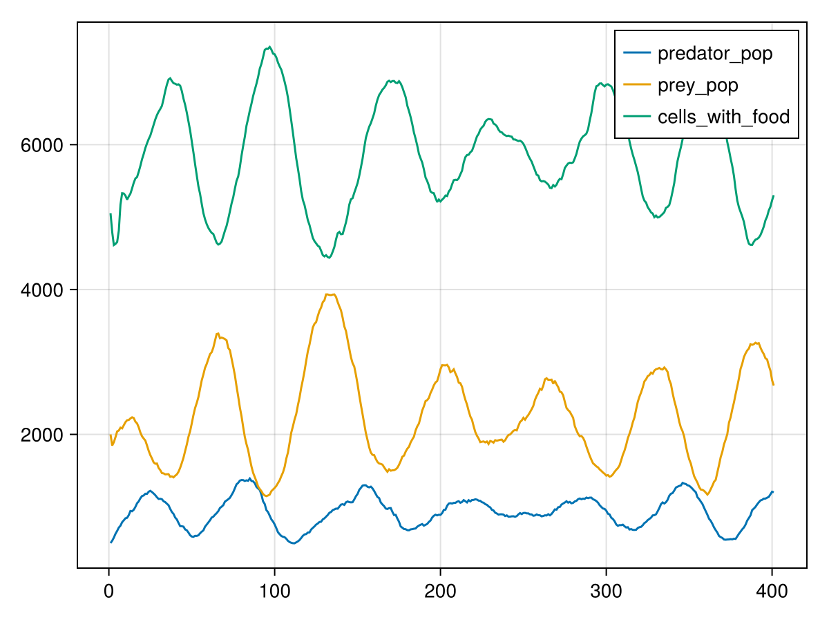

Spatial distribution

To visualize the spatial information we can use heatmap in combination with the Vahana's calc_raster function. E.g. the number of Position{Prey} edges connected to a cell give us the number of Prey individuals currently on that cell.

It would be nice to have a colorbar for the heatmaps so we define a small helper function that can be used in a pipe.

function add_colorbar(hm)
    Makie.Colorbar(hm.figure[:,2], hm.plot)
    hm
end;

Predators Positions

calc_raster(ppsim, :raster, Int64, [ Position{Predator} ]) do id
    num_edges(ppsim, id, Position{Predator})
end |> heatmap |> add_colorbar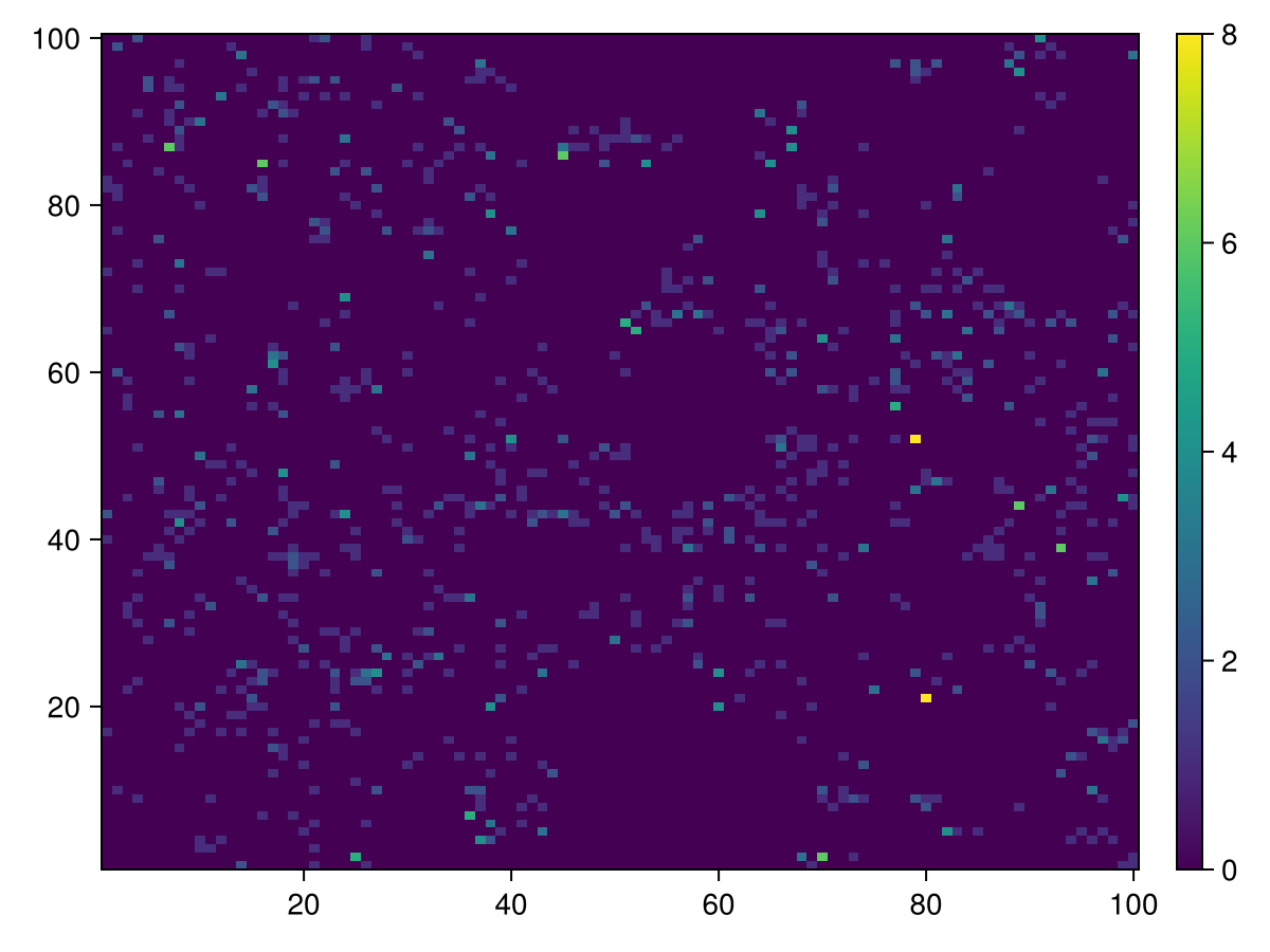

Prey Positions

calc_raster(ppsim, :raster, Int64, [ Position{Prey} ]) do id
    num_edges(ppsim, id, Position{Prey})
end |> heatmap |> add_colorbar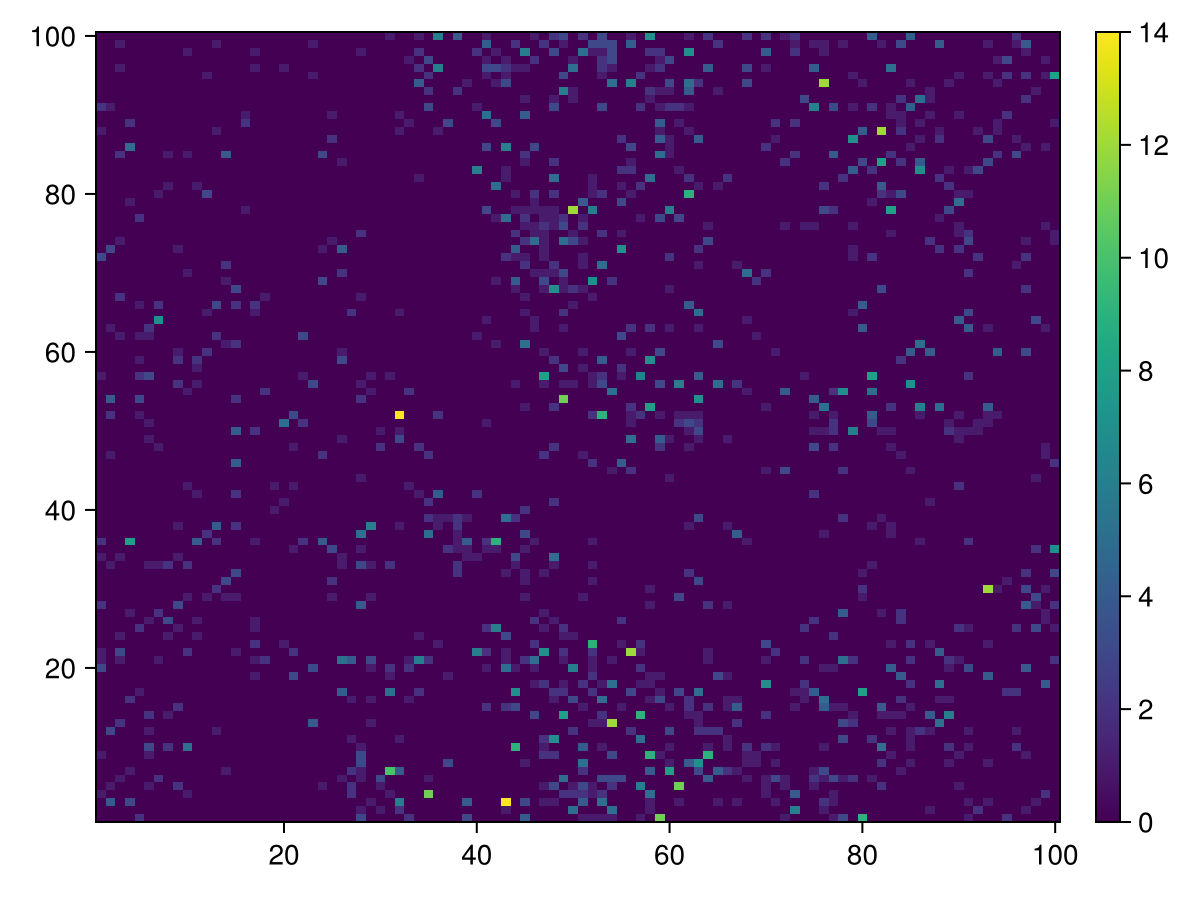

Cells that contains food

calc_raster(ppsim, :raster, Int64, [ Cell ]) do id
    agentstate(ppsim, id, Cell).countdown == 0
end |> heatmap |> add_colorbar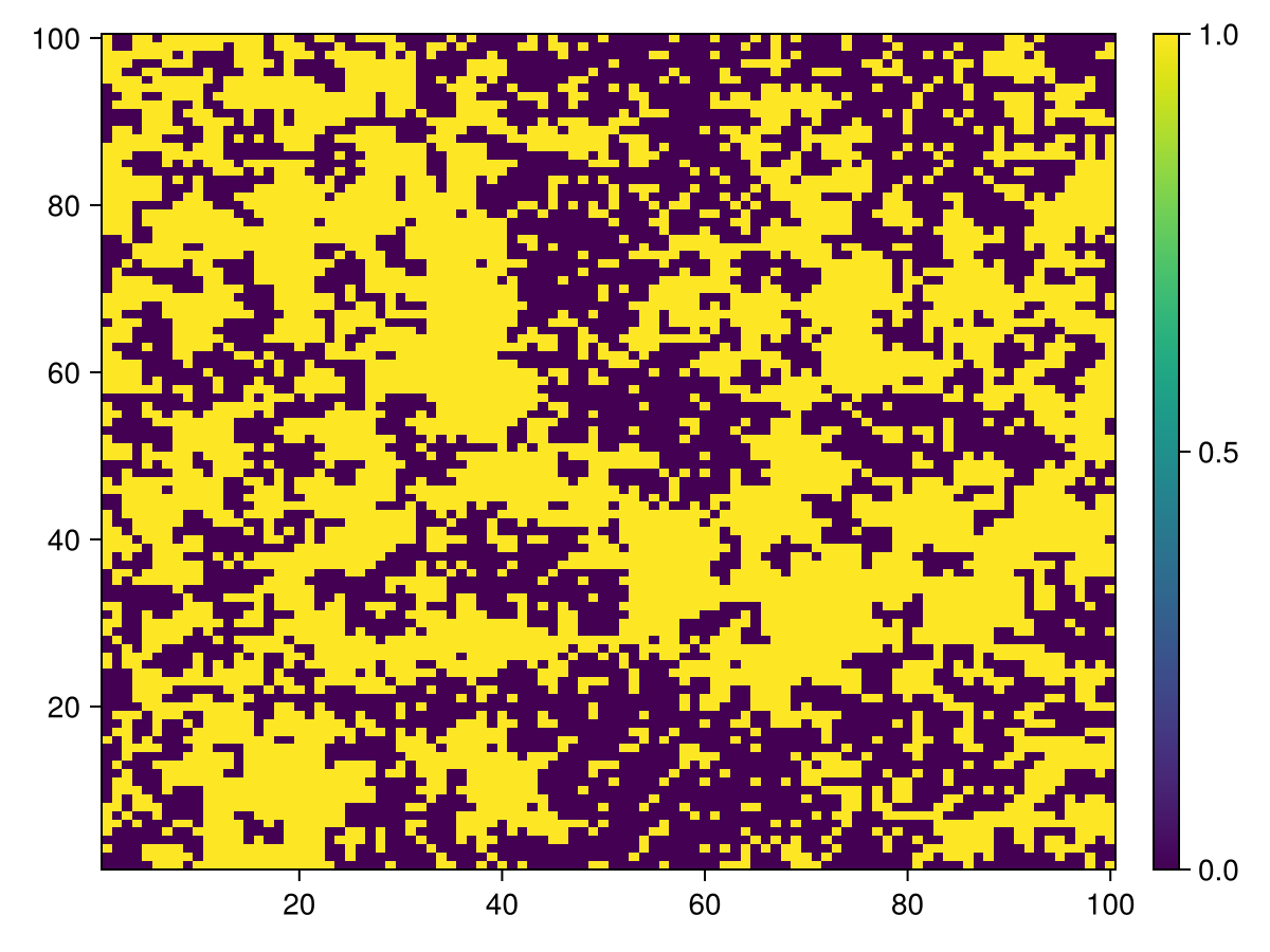

Finish the Simulation

As always, it is important to call finish_simulation at the end of the simulation to avoid memory leaks.

finish_simulation!(ppsim);

This page was generated using Literate.jl.