Utilizing Graphs.jl

Goal

This tutorial illustrates how to integrate graphs that support the AbstractGraph interface from the Graphs.jl package into a Vahana simulation and the visualization support for Vahana graphs.

For this purpose, we implement the opinion dynamics model of Hegselmann and Krause (2002). An alternative implementation of the same model using the Agents.jl package can be found here.

Agent and Edge Types

using Vahana, Statistics

We have a finite number $n$ of agents, where the state of the agents are a real number $x_i(t)$ in the [0,1] interval which represents the opinion of that agent.

struct HKAgent
    opinion::Float64
end

This time we have only one network that determine the agents that will be considered when an agent updates its opinion.

struct Knows end

Beside these two types there is a confidence bound $\epsilon > 0$, opinions with a difference greater than $\epsilon$ are ignored by the agents in the transition function. All agents have the same confidence bound, so we introduce this bound as a parameter.

const hkmodel = ModelTypes() |>
    register_agenttype!(HKAgent) |>
    register_edgetype!(Knows) |>
    register_param!(:ϵ, 0.02) |> # the confidence bound
    create_model("Hegselmann-Krause");

Edgetype Knows is a struct without any field, so you can increase the
performance by setting the :Stateless hint. You can also
calling detect_stateless() before calling register_edgetype!,
then the :Stateless hint will be set automatically for structs without
a field.

Adding a Graph

Vahana allows adding SimpleGraphs and SimpleDiGraphs from the Graphs.jl package via the add_graph! function. So it is possible to use e.g. SNAPDatasets to run the opinion model on real datasets, or the SimpleGraphs module from Graphs.jl to create synthetic graphs.

We demonstrate here both use cases and are creating a separate simulation for each one.

const cgsim = create_simulation(hkmodel);
const snapsim = create_simulation(hkmodel)

Model Name: Hegselmann-Krause
Simulation Name: Hegselmann-Krause
Agent(s):
	 Type HKAgent with 0 agent(s)
Edge(s):
	 Type Knows with 0 edge(s) for 0 agent(s)
Parameter(s):
	 :ϵ : 0.02
Still in initialization process!.

SimpleGraphs

First we will show how we can add a synthetic graph. For this we need to import the SimpleGraphs module. Since there are many functions in the Graphs.jl package with the same name as in Vahana (e.g. add_edge!), it is advisable to import only the needed parts of Graphs.jl instead of loading the whole package via using Graphs.

import Graphs.SimpleGraphs

We want to add a complete graph, where each agent is connected with all the other agents, like in the Agents.jl implementation. We can create such a graph via SimpleGraphs.complete_graph.

g = SimpleGraphs.complete_graph(50)

{50, 1225} undirected simple Int64 graph

Vahana needs the information how to convert the nodes and edges of the SimpleGraphs object to the Vahana structure. This is done by the constructor functions in the third and forth arguments of add_graph!. We do not need the Graph.vertex and Graph.edge arguments of this constructor functions, but for other use cases e.g. for bipartite graphs, it would be possible to create agents of different types depending on this information.

const agentids = add_graph!(cgsim,
                            g,
                            _ -> HKAgent(rand()),
                            _ -> Knows());

Each agent also adds its own opinion to the calculation. We can use the ids returned by the add_graph! functions for this.

foreach(id -> add_edge!(cgsim, id, id, Knows()), agentids)

finish_init!(cgsim)

SNAPDataset.jl

The SNAPDataset.jl package delivers Graphs.jl formatted datasets from the Stanford Large Network Dataset Collection.

using SNAPDatasets

With this package we can use the loadsnap function to create the graph that is then added to the Vahana graph, e.g. in our example the facebook dataset.

const snapids = add_graph!(snapsim,
                           loadsnap(:facebook_combined),
                           _ -> HKAgent(rand()),
                           _ -> Knows());

Again each agent adds its own opinion to the calculation.

foreach(id -> add_edge!(snapsim, id, id, Knows()), snapids)

finish_init!(snapsim)

The Transition Function

Opinions are updated synchronously according to

\[\begin{aligned} x_i(t+1) &= \frac{1}{| \mathcal{N}_i(t) |} \sum_{j \in \mathcal{N}_i(t)} x_j(t)\\ \textrm{where } \quad \mathcal{N}_i(t) &= \{ j : \| x_j(t) - x_i(t) \| \leq \epsilon \} \end{aligned}\]

So we first filter all agents from the neighbors with an opinion outside of the confidence bound, and then calculate the mean of the opinions of the remaining agents.

function step(agent, id, sim)
    ϵ = param(sim, :ϵ)

    opinions = map(a -> a.opinion, neighborstates(sim, id, Knows, HKAgent))

    accepted = filter(opinions) do opinion
        abs(opinion - agent.opinion) < ϵ
    end

    HKAgent(mean(accepted))
end;

We can now apply the transition function to the complete graph simulation

apply!(cgsim, step, HKAgent, [ HKAgent, Knows ], HKAgent)

Model Name: Hegselmann-Krause
Simulation Name: Hegselmann-Krause
Agent(s):
	 Type HKAgent with 50 agent(s)
Edge(s):
	 Type Knows with 2500 edge(s) for 50 agent(s)
Parameter(s):
	 :ϵ : 0.02

Or to our facebook dataset

apply!(snapsim, step, HKAgent, [ HKAgent, Knows ], HKAgent)

Model Name: Hegselmann-Krause
Simulation Name: Hegselmann-Krause
Agent(s):
	 Type HKAgent with 4039 agent(s)
Edge(s):
	 Type Knows with 180507 edge(s) for 4039 agent(s)
Parameter(s):
	 :ϵ : 0.02

Creating Plots

Finally, we show the visualization possibilities for graphs, and import the necessary packages for this and create a colormap for the nodes.

import CairoMakie, GraphMakie, NetworkLayout, Colors, Graphs, Makie

Since the full graph is very cluttered and the Facebook dataset is too large, we construct a Clique graph using Graphs.jl.

const cysim = create_simulation(hkmodel) |> set_param!(:ϵ, 0.25);

const cyids = add_graph!(cysim,
                         SimpleGraphs.clique_graph(7, 8),
                         _ -> HKAgent(rand()),
                         _ -> Knows());


foreach(id -> add_edge!(cysim, id, id, Knows()), cyids)

finish_init!(cysim);

Vahana implements an interactive plot function based on GraphMakie, where agents and edges are given different colors per type by default, and the state of each agent/edge is displayed via mouse hover actions.

vp = create_graphplot(cysim)

figure(vp)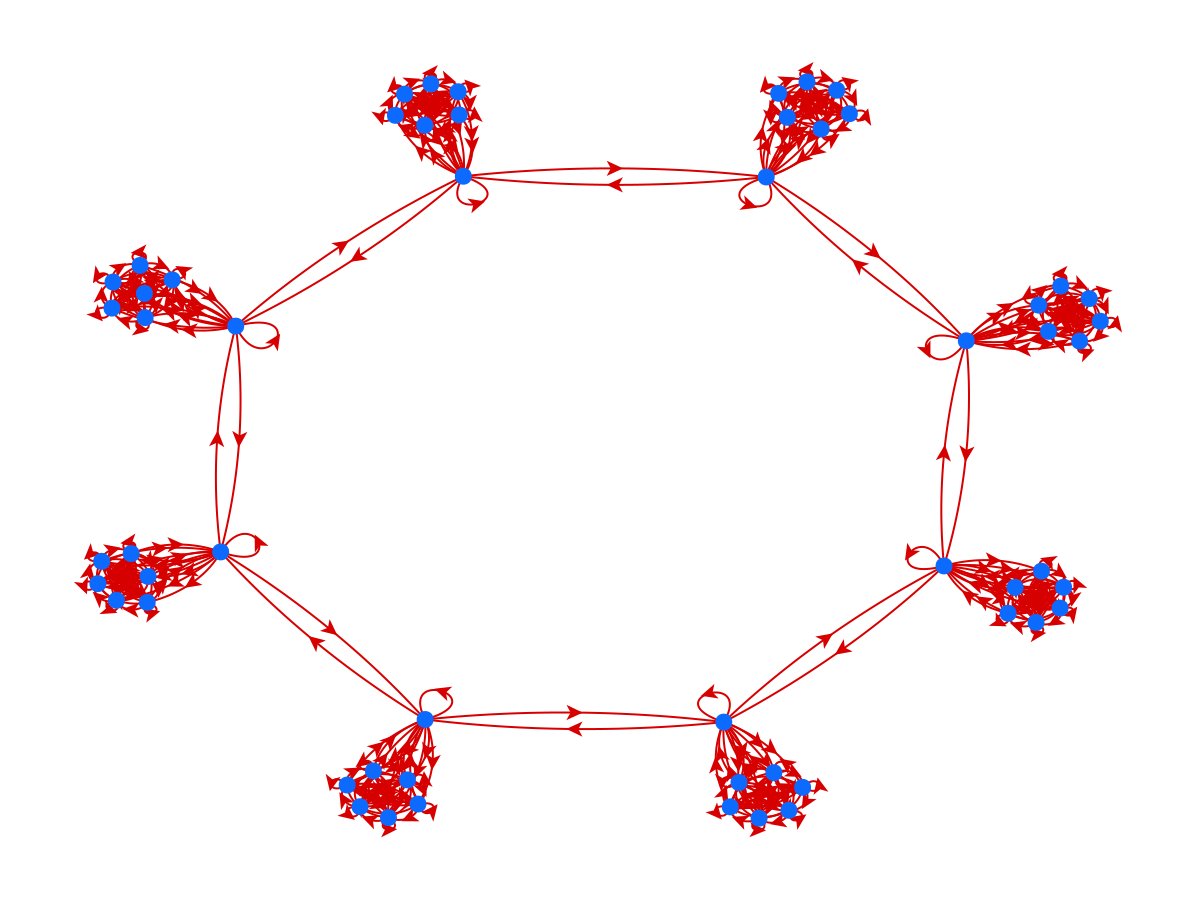

To modify the created plot, the Makie figure, axis and plot, can be accessed via the methods figure, axis and plot. This allows us to modify the graph layout and to remove the decorations.

Vahana.plot(vp).layout = NetworkLayout.Stress()

Makie.hidedecorations!(axis(vp))

figure(vp)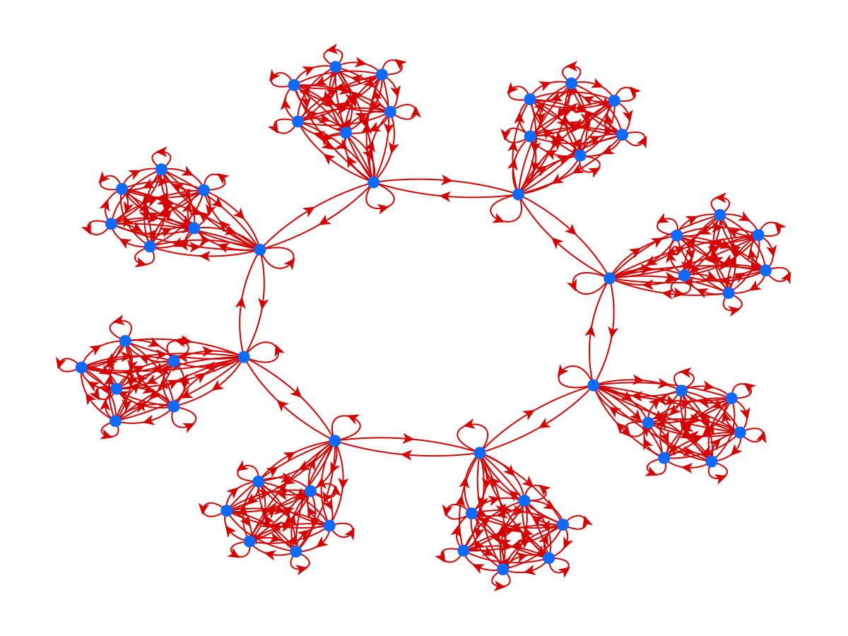

To visualize the agents' opinions, we can leverage Vahana's integration with Makie's plotting capabilities. Instead of directly modifying the node_color property of the Makie plot, we can define custom visualization functions. These functions, which can have methods for different agent and edge types, are used by create_graphplot to determine various properties of nodes and edges in the plot.

This approach not only allows for more dynamic and type-specific visualizations but also supports interactive plots when using GLMakie as the backend. We'll define a function called modify_vis that specifies how different elements should be displayed. This function will be passed to create_graphplot via the update_fn keyword argument.

colors = Colors.range(Colors.colorant"red", stop=Colors.colorant"green", length=100)


modify_vis(state::HKAgent, _ ,_) = Dict(:node_color => colors[state.opinion * 100 |> ceil |> Int],
                                       :node_size => 15)

modify_vis(_::Knows, _, _, _) = Dict(:edge_color => :lightgrey,
                                     :edge_width => 0.5);

function plot_opinion(sim)
    vp = create_graphplot(cysim,
                          update_fn = modify_vis)
    Vahana.plot(vp).layout = NetworkLayout.Stress()
    Makie.hidedecorations!(axis(vp))
    Makie.Colorbar(figure(vp)[:, 2]; colormap = colors)
    figure(vp)
end;

And now we can plot the initial state

plot_opinion(cysim)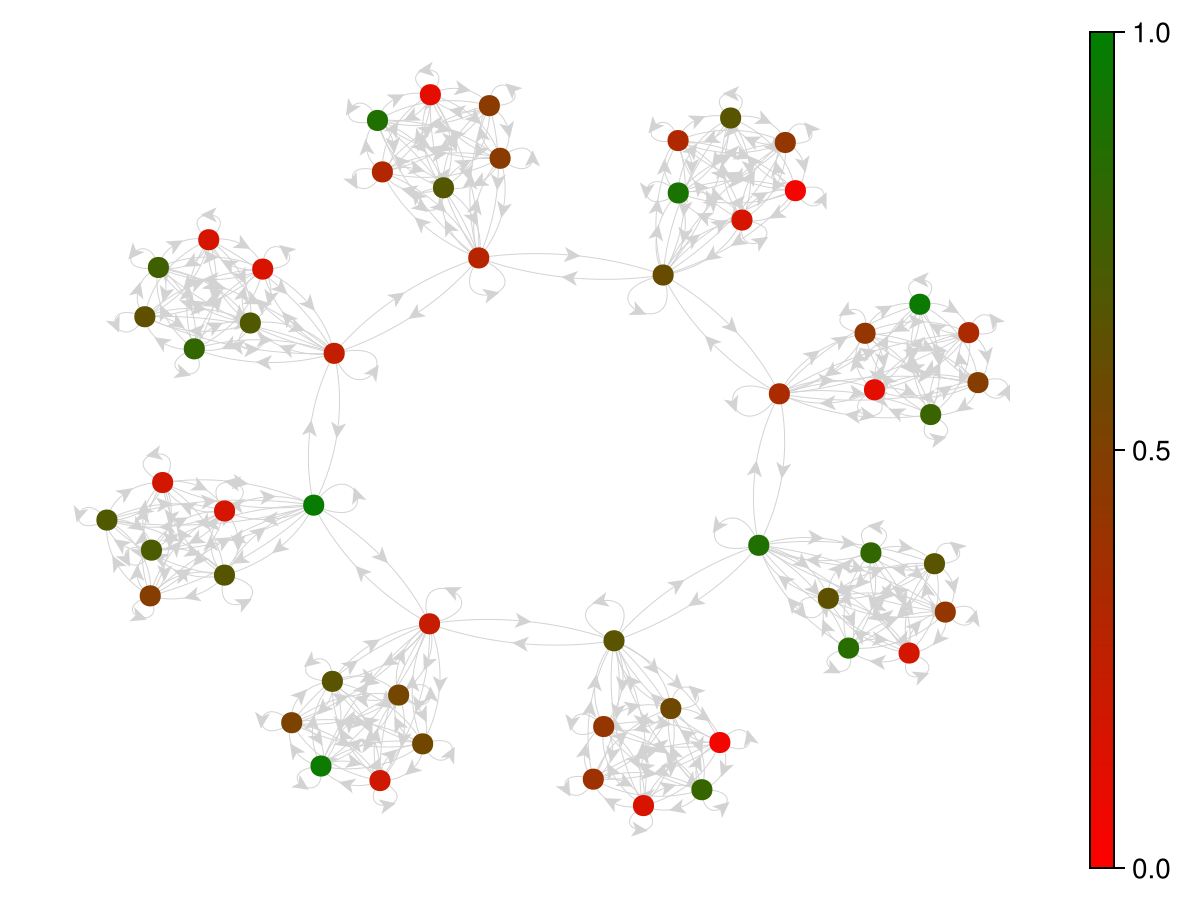

And then the state after 500 iterations

for _ in 1:500
    apply!(cysim, step, [ HKAgent ], [ HKAgent, Knows ], [ HKAgent ])
end

plot_opinion(cysim)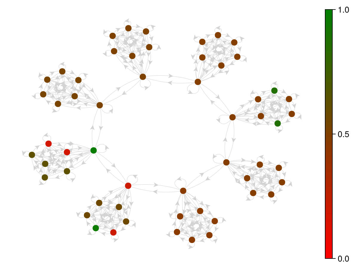

Finish the Simulation

As always, it is important to call finish_simulation at the end of the simulation to avoid memory leaks.

finish_simulation!(cysim);

This page was generated using Literate.jl.